Click on the image to run the program with Java WebStart
Press here to run the program in the browser

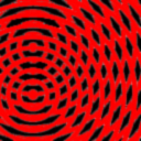
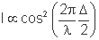
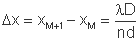
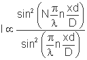
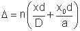
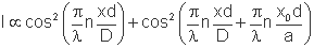
Young's experiment

This applet shows Young interferences resulting from the interaction of a certain number of waves. When using a single extended source or two point sources, spatial coherence can be studied as well.

"Plane wave" window

In this window you can study Young's interference fringes resulting from the superposition of several point sources. The schema shown on the upper left side shows an incident plane wave on a plane containing N slits separated by distance d, which are normal to the plane of the drawing. Each of these holes gives rise to secondary coherent waves, as indicated by Huygens' theorem. When observing their superposition on a plane that is a distance D from the slits, we can see interference fringes normal to the drawing plane. These fringes are shown on the upper right side of the window.

Let us first consider the case of N=2 (double slit): if we assume that the amplitude of both waves is equal for any point within the observation plane, the intensity of the fringes is:

where λ is the wavelength of light (in the vacuum) and Δ is the optical path difference between the waves coming from the two slits. If we take the approximation

(observation plane far enough away), the optical path difference is:

where n is the refraction index of the medium where the waves propagate and x is an axis parallel to the line joining them. We should remember that d is the separation between the slits and D is the distance between the plane containing them and the observation plane.

Whenever the optical path difference is an integer multiple of the wavelength, constructive interference will take place. If n, d and D are fixed, this depends only on the x-coordinate, which explains why interference fringes are observed. The locations of the several maxima are:

with M being an integer value. The distance between maxima (fringe spacing) is:

Between every two maxima there is a minimum, for which there is destructive interference and the intensity falls to zero. The applet gives the distance between maxima and minima, which is the same in the case of N=2.

You can also change the system parameters and see the evolution of the corresponding interference image, whose color is in accordance with the selected wavelength. By pressing the "Graphic" button, the intensity profile is shown. When pressing the "Image" button, the fringe pattern is shown again. This is by default on a linear scale, which is indicated by the "Linear intensity on" button. After pressing it, the intensity appears on a logarithmic scale and the button label changes to "Logarithmic intensity on". The graphics window width is automatically modified to assure that maxima and minima are plotted with a good resolution.

In the general case of N>2, the intensity of the fringes becomes:

This function has a series of main maxima for which the intensity is maximum, separated the same distance Δx as before. Every two main maxima there are N-2 secondary maxima and N-1 minima, of null intensity, having a separation:

All these general formulae reduce to the formula for the "double slit" case N is replaced by 2.

"Spatial coherence" window

In this window you can see the dependence of the visibility of the interference fringes for Young's experiment (double slit case) on the characteristics of the light source, in order to study the spatial coherence phenomenon. The visibility factor is defined as:

where I_M and I_m is the fringe maximum and minimum intensity, respectively.

In the "plane wave" window, slits were illuminated by a plane wave. Now, there are several options for the light source:

• One point source located a certain distance x₀ away from the slits (x=0): this corresponds to the previous case but now the path length difference has an additional term:

  

  where a is the distance between the plane of the source and the slits' plane. Therefore, the fringes are not centered at x=₀, but at:

  

  for which the path length difference vanishes. If the source is placed above the center, the fringes are displaced to the opposite side, downwards (to the right of the plot). In any case, the visibility is V=1 as I_m=0.

• Two point sources separated a certain distance x₀: the resulting intensity is the sum of the contribution of each source, which give fringes centered at different points:



This gives place to a fringe structure having the same fringe spacing as in the case of a single source, but having a poorer contrast. The visibility factor is:



• A single extended source: the intensity distribution can be found by superposing (integrating) the resulting fringes along the entire source extension ΔS:



As before, the fringe spacing remains the same, whereas the fringe visibility becomes: