Life tables - R programming

Mercedes Ayuso, Montserrat Guillén and Ana María Pérez-Marín

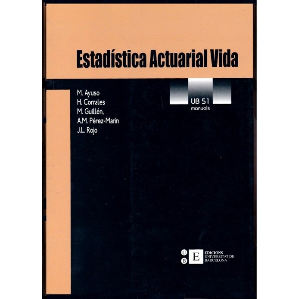
• Ayuso, M., Corrales, H., Guillén, M., Pérez-Marín, A.M. and Rojo, J.L. (2007) Actuarial statistics for life insurance [Estadística actuarial vida], Publicacions i Edicions de la Universitat de Barcelona

DATA DESCRIPTION

Name	Content description
H91_09_DEAD.csv	Men death rates in Spain from 1991 to 2009. Source: INE.
H91_09_EXPO.csv	Men exposure to risk in Spain from 1991 to 2009. Source: INE.
Mx1_x1SPAIN.txt	Death rates in Spain since 1908 to 2006, from 0 years to +110.
Exposures_1x1SPAIN.txt	Exposure to risk in Spain since 1908 to 2006, from 0 years to +110.

Download H91_09_DEAD.csv data set here.	Download H91_09_EXPO.csv data set here.
Download Mx_1x1SPAIN.txt data set here.	Exposures_1x1SPAIN.txt data set here.

ANALYSIS OF GROSS MORTALITY RATES AND BASIC LIFE TABLES

In this example we use data from the Human Mortality database and from the Spanish Statistics Institute (INE).

Namely, the script below shows how to read and plot gross death rates in a logarithmic scale and data on the exposure to the risk of mortality for Spain.
We also plot the life expectancy at birth and from 65 years old for men and women. Additionally, we also plot death rates for male older than 65 and the life expectancy at different ages. Finally, we print a basic life tables for Spain.

- Script

Download the R script here.

Download results here.

DATA CLEANING OF GROSS MORTALITY RATES

We show different graphical methods to represent mortality rates as a function of age and calendar year.

In this way, mortality improvement over calendar time is shown by using different types of plots.
Then, data cleaning of gross mortality rates is carried out by using alternative techniques (outlier imputations, smoothing techniques, linear extrapolation for advanced ages). More details can be found in Actuarial statistics for life insurance.

- Script

Download the R script here.

Download results here.

GRADUATION OF MORTALITY CURVES-STATIC

We show how to fit a Gompertz model to the mortality experience in one calendar year (static mortality curve):

\begin{equation} l_x = Kg^{C^{x}}, \,\,\,\,\,\,\,\,\,\,\,\, K > 0, \,\, 0 < g < 1, \,\, C>1. \\ lnl_x = lnK + C^{x}lng \,\,\,\,\,\,\,\,\,\,\,\,\,\,\,\,\,\,\,\,\,\,\,\,\,\,\,\,\,\,\,\,\,\,\,\,\,\,\,\,\,\,\,\,\,\,\,\,\,\,\, \end{equation} \begin{equation} q_x = 1-g^{C^{x}(C-1)} \,\,\,\,\,\,\,\,\,\,\,\,\,\,\,\,\,\,\,\,\,\,\,\,\,\,\,\,\,\,\,\,\,\,\,\,\,\,\,\,\,\,\,\,\,\,\,\,\,\,\,\,\,\,\,\,\,\,\,\,\,\,\,\,\,\,\,\\ ln(1-q_x) = C^x[(C-1)lng] \,\,\,\,\,\,\,\,\,\,\,\,\,\,\,\,\,\,\,\,\,\,\,\,\,\,\,\,\,\,\,\,\, \end{equation} \begin{equation} \mu_x = -lnglnCC^{x} \,\,\,\,\,\,\,\,\,\,\,\,\,\,\,\,\,\,\,\,\,\,\,\,\,\,\,\,\,\,\,\,\,\,\,\,\,\,\,\,\,\,\,\,\,\,\,\,\,\,\,\,\,\,\,\,\,\,\,\,\,\,\,\,\,\,\,\\ ln\mu_x = A + Bx \,\,\,\,\,\,\,\,\,\,\,\,\,\,\,\,\,\,\,\,\,\,\,\,\,\,\,\,\,\,\,\,\,\,\,\,\,\,\,\,\,\,\,\,\,\,\,\,\,\,\,\,\,\,\,\,\,\,\,\,\,\,\,\,\, \\ A = ln(-lnClng), B = lnC \,\,\,\,\,\,\,\,\,\,\,\,\,\,\,\,\,\,\,\,\,\,\,\,\,\,\,\,\,\,\,\,\, \end{equation}
where l_x are the individuals alive at age x, q_x is the death rate at age x and μ_x is the force of mortality at age x. K,g and C are parameters of the model.

- Script

Download the R script here.

Download results here.

ESTIMATION AND PREDICTION BY USING THE LEE-CARTER METHOD

In this example, we show how to estimate a Lee-Carter method, introduced by Lee and Carter (1992), to the mortality experience for spanish men older than 65 (time period 1975-2006). Additionally, the Lee-Carter prediction of the life expectancy is also carried out.

\begin{equation} ln\hat\mu_x(t) = ln\mu_x(t) + \epsilon_x(t), \,\,\,\,\,\,\,\,\,\,\,\,\,\,\,\,\,\,\,\,\,\,\,\,\,\,\,\,\,\,\,\,\,\,\,\, \\ \mu_x(t) = exp(\alpha_x + \beta_{x}k_{t}), \,\,\,\,\,\,\,\,\,\,\,\,\,\,\,\,\,\,\,\,\,\,\,\,\,\,\,\,\,\,\,\,\,\,\,\,\,\,\, \\ \epsilon_x(t) \sim \mathcal{N}(0,\sigma^2) \,\,\,\,\,\,\,\,\,\,\,\,\,\,\,\,\,\,\,\,\,\,\,\, \end{equation}

- Script

Download the R script here.

Download results here.

ESTIMATION OF THE LTC MODEL EXTENSIONS AND MODEL SELECTION

We fit and compare three alternative models to mortality data for men, 1991-2009 (Spain). The three models are:

M1: Lee-Carter
M5: CBD model
M7: Second generalization of the CBD model

- Script

Download the R script here.

REFERENCES

[1] Ayuso, M., Corrales, H., Guillen, M. et al. (2001) Estadística Actuarial Vida. Barcelona: Universitat de Barcelona.

[2] Brouhns, N. and Denuit, M. (2002) Risque de longévite et rentes viagères I. Evolution de la mortalité en Belgique de 1880 à nos jours. Belgian Actuarial Bulletin, Vol.2, No. 1, 26-48.

[3] Brouhns, N. and Denuit, M. (2002) Risque de longévite et rentes viagères II. Tables de mortalité prospectives pour la population belge. Belgian Actuarial Bulletin, Vol.2, No. 1, 49-63.

[4] Brouhns, N. and Denuit, M. (2002) Risque de longévite et rentes viagères III. Elaboration de tables de mortalité prospectives pour la population assurée belge, et évaluation du coût de l'antisélection. Belgian Actuarial Bulletin, Vol.2, No. 1, 64-72.

[5] Cairns, A., Blake, D., Dowd, K. et al. (2009) A Quantitative Comparison of Stochastic Mortality Models Using Data from England & Wales and the United States. North American Actuarial Journal, Vol.13, No. 1, 1-35.

[6] Delwarde, A. and Denuit, M. (2003) Importance de la période d'observation et des âges considérés dans la projection de la mortalité selon la méthode de Lee-Carter. Belgian Actuarial Bulletin, Vol.3, No. 1, 1-21.

[7] Haberman, S. and Pitacco, E. (1999) Actuarial Models for Disability Insurance. United States: Cahpman & Hall/CRC.

[8] Knorr, F.E. (1984) Multidimensional Whittaker-Henderson graduation.Transactions of Society of Actuaries, Vol.36, 213-255.

[9] Lee, R. D. and Carter, L. (1992) Modeling and Forecasting the Time Series of U.S. Mortality. Journal of the American Statistical Association 87, 659-671.

[10] Pitacco, E., Denuit, M. et al. (2009) Modelling Longevity Dynamics for Pensions and Annuity Business. United States: Oxford University Press.

[11] Renshaw, A.E. and Haberman, S. (2003) On the forecasting of mortality reduction factors. Insurance: Mathematics and Economics, Vol.32, No. 3, 379-401.