In this tutorial you will find a set of instructions describing how to perform Dynamic Undocking (DUck) and analyze the results. The procedure will be supported by the example of cationic trypsin (PDB: 2AYW) and a library of fragments lig_lib.mdb, previously docked to the protein with rDock. All the files required for the simulation can be downloaded here.
More information about Dynamic Undocking can be found here: Dynamic undocking and the quasi-bound state as tools for drug discovery
Getting Started
To perform DUck smoothly you need fulfill listed requrements (software and hardware):
- Molecular Operating Environment (MOE)
- Download MOE (versions 2015, 2016 and above). License required.
- Open MOE installer and follow instructions.
- Molecular Dynamics Package (AMBER)
- Download Amber and AmberTools (version 16) from their website (http://ambermd.org/) and follow the installation instructions for your platform.
- AmberTools is free but you will need a license for running Amber.
- Make sure AmberTools is installed locally and their binaries are visible (adapt $PATH variable if needed) so MOE can run them.
- PyMol
- Download the PyMol Molecular Viewer at http://www.pymol.org/. Click on “Download”. On the next page, fill out the information according to your status.
- Follow the instructions to download and install PyMol.
- R
- Download R software from at https://cran.r-project.org/ for your platform.
- Follow the instructions and make sure that R and Rscript binaries are visible during production stage.
- DUck scripts
- Download the public DUck scripts from https://github.com/CBDD/duck.
- Hardware
- Computer workstations with Linux or MAC OS for DUck preparations.
- Computational cluster with Linux-based OS for parallelization and GPUs for MD simulations (DUck is compatible with SGE and SLURM queueing systems).
It’s better to perform simulation on a server (however it’s possible to run it locally). The rest of steps (preparation of system) can be performed locally. It can make a difference in your package distribution.
DUck is distributed as a package of scripts available here and also on github. After unpacking, preparation of DUck is pretty straightforward – set the environmental variable to proper directory with duck.svl script:
For MOE2015:
tar -xzf duck.tar.gz
cd duck/
export MOE_SVL_LOAD=$(pwd)
echo export MOE_SVL_LOAD=$(pwd) >> ~/.bashrc
For MOE2016 and newer versions:
tar -xzf duck.tar.gz
Make sure all scripts are located in $HOME/moefiles/svl directory
Key interaction identification
The first and essential step is the identification of the key atom in the receptor that forms hydrogen bond with the ligand. DUck will force the rupture of this interaction. The atom of reference must form hydrogen bond with all (or most) known ligands. For well-known systems, like the one used here, it can be identified from a structural superimposition of all the available protein-ligand complexes. On novel binding sides, it may be identified with a hot spot identification method.
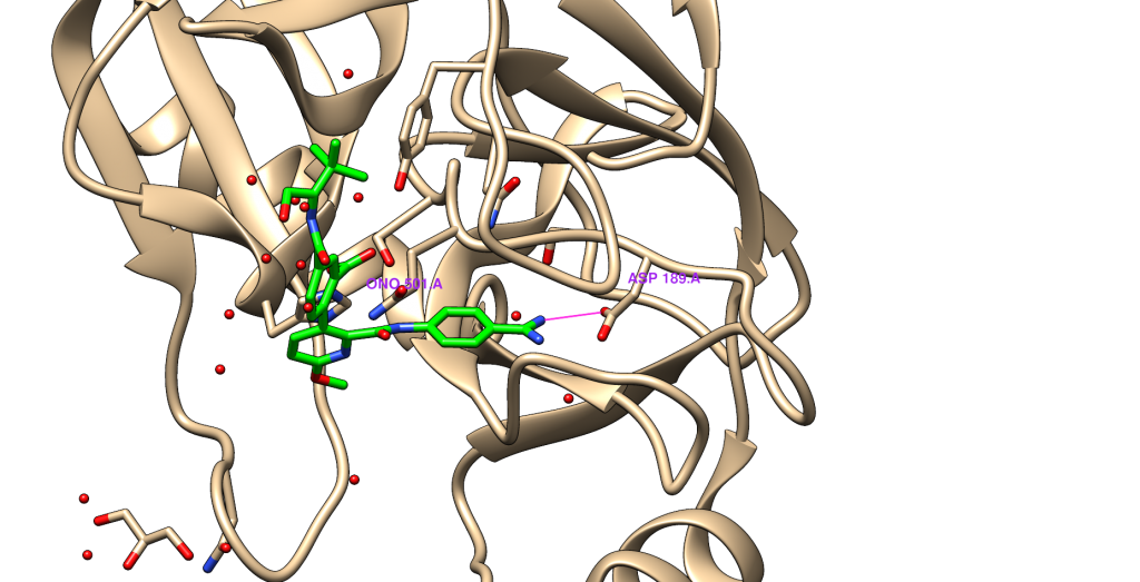
In trypsin the key hydrogen bond is formed between oxygen of Asp189 and corresponding nitrogen atom in the ligand. As atom of reference we will use one of the oxygens of carboxyl group of that residue.
System preparation
Protein chunk preparation
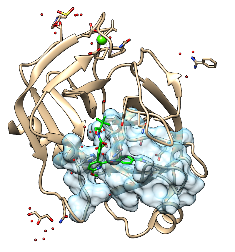
One of the most important steps in system preparation is chunk selection. “Chunk” is a minimal subset of residues that preserve the local environment around the key hydrogen bond. Selection of residues is essential for the accurate result of Dynamic Undocking, thus very careful visual inspection is required. Excess residues will slow down calculation and can potentially block the ligand from leaving the pocket, resulting in very high WQB values that do not reflect the strength of the hydrogen bond. An incomplete structure will result in artificially high solvent exposure, which will render the hydrogen bond more labile and cause to underestimate WQB value. The following steps describe chunk preparation process:
- If Dynamic Undocking was preceded by docking, it is best to use the same protonated structure. In any other case, eg. X-ray structure, the protein structure must be prepared by protonation with a standard protocol implemented in MOE software, or other protonation methods. Essential water molecules for complex stability must be identified and preserved in the structure. The rest of water molecules, ions and other ligands must be removed from the system.
- Initially, chunk is created by selecting residues within 6-7 Å of the atom of reference. To complete the base selection further, visual inspection is needed. Additional residues must be added, based on following rules:
- Residues important for protein-ligand interaction,
- Residues blocking channels in the structure, preventing solvent molecules from accessing the key H-Bond through holes created when carving the chunk out of the protein matrix
- Residues connecting parts of chunk, if sequence gap between two selected parts of the protein is less than 3 residues.
- Preserve interstitial water molecules that may be essential for complex stability.
- Unselected residues are eliminated. Typically, this causes polypeptidic chains to split into separate chains. To prevent charged ends and unnatural electrostatic forces, chains must be capped with acetyl and N-methyl groups.
- Final structure has to be saved in MOE format, with names of residues adjusted to AMBER force field.
In this example we have used cavity composed of the closest residues to the OD2 atom in Asp189. The structure was divided into separate chains and the ends of the chains were acetylated or N-methylated. Then the structure was protonated and, if needed, clashes were removed. Appropriate structure, prepared using MOE, is provided in the file (trypsin_chunk.pdb).
Ligand library preparation
Except for the receptor model, a set of properly oriented ligands is required (docking poses or superimposed X-ray geometries). Library of ligands can be obtained using any docking procedure.
For this example we used the library of 10 ligands, produced by docking in rDock (lig_lib.mdb). The library was inspected by MOE and the structures were protonated (washed) and saved into field called mol (this exact name is required to complete the next step). Additionally, to check if the next step will be processed smoothly, partial charges were assigned using AM1-BCC method. In case of clash, the structure has to be modified. Otherwise the SVL script will crash. Once you have prepared your ligand DB save it in *.mdb format.
Simulation preparation in MOE
The next step of the procedure is done automatically by MOE SVL script, which performs following steps:
- Calculates AM1-BCC charges for the ligand
- Assigns parm@Frosst atom types and non-bonded parameters to the ligand
- Identifies the ligand atom that is hydrogen-bonded to the protein’s reference atom (based on the distance and type of atom)
- Writes input and execution files to carry out the MD simulations with AMBER
- Calls AMBER’s tLeap to generate valid topology and coordinate files for each individual receptor-ligand complexes.
The script creates series of files that will perform the Dynamic Undocking, which can be later transfer to server and used to perform steered molecular dynamics. For the protein AMBER force field 99SB is used. Each system is placed in cuboid box spanning at least 12 Å more than the furthest atom in each direction. The box is then filled with TIP3 water molecules to create periodic boundary conditions. When needed, Na+ or Cl– are added to force the neutrality of the whole system.
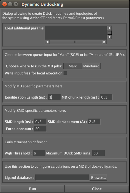
In our example we loaded the structure of the receptor to MOE and marked the atom of the receptor that makes key interaction. Then the SVL script (duck.svl) was loaded. It opens a window in which you can edit parameters of the DUck simulation:
- Field “load additional params” is useful in cases of structures of ligand with metal ions (Zinc, Calcium or Manganese), since the force field parameters for metal ions are not included.
- The other variable is a queue system that will be used for the simulation, either SGE (Marc) or SLURM (Minotauro). However, it is also possible to run calculations on local UNIX. Appropriate *.sh files are created by marking the box.
- In the next section we can modify MD parameters:
- equilibration length (default 1 ns)
- free chunk MD length (500 ps) – length of molecular dynamic between consecutive SMD simulations in order to generate different starting points for SMD.
- The next section is for modifying steered molecular dynamics parameters:
- length of the simulation (default 500 ps),
- SMD displacement (Å) (default 2.5) – the distance that the ligand is going to be displaced, starting at the distance of 2.5 Å from reference atom in ligand,
- force constant of the spring that is pulling ligand out of the pocket (default 50 kcal/mol Å2).
- In the “Early termination definition” section we can:
- establish threshold of work, below which calculations will be terminated (default 6 kcal/mol). Optimal value depends on the system and set of ligands. For most of cases the threshold 6 kcal/mol is sufficient. If you find that, for your system, known ligands break with weak forces, a lower WQB threshold may be necessary.
- set the maximum number of calculations (default 50).
- In the last section we selected database with prepared ligands. Before running the calculation make sure that tleap (ambertools) can be called from the terminal.
Script creates a series of files, essential for SMD:
- submit_duck_smd_gpu.csh – calls *.q files in subdirectories and submits SMDs to the queue system.
- getWqbValues.R – R script that calculates the value of WQB.
- duck_template_gpu.q and duck_template_gpu_325K.q – submit the SMD to queue system.
The rest of files are collected in LIG_target_* folders, separate for every ligand:
- equil.q, md*.q – equilibration file submits a job with equilibration of the system to the server queue, the md*q files submit jobs that perform the SMDs (both in 300 K and 325 K), preceded by 1 ns of unbiased dynamics, to increase the sampling.
- 1_min.in, 2_eq.in, 3_eq_200.in, 3_eq_250.in, 3_eq_300.in, 4a_eq.in, 4b_eq.in – contain the parameters for the equilibration stage.
- md.in – contain the parameters for the molecular dynamics stage.
- duck.in and duck_325K.in – contain the parameters for the steered molecular dynamics stage in both 300 and 325 K.
- dist_md.rst – include identification number of atoms that form hydrogen bond and the parameters of restrains applied to ligand during MD.
- dist_duck.rst – include identification number of atoms that form hydrogen bond, the initial and final distance between key atom in the receptor and end of the string that applies the force to the ligand during the SMD.
- lib/ – directory gathers files with the solvated system in the simulation box. Ions are added to force the neutrality of the system.
Dynamic Undocking
In order to equilibrate the system the following steps are executed:
- Energy minimization for 1000 cycles.
- Assignment of random velocities at 100 K and gradual warming to to 300 K for 400 ps in the NTV ensemble
- Equilibration of the system for 1 ns in the NPT ensemble (1 atm, 300 K). This phase was spited into two stages – 10 000 and 490 000 steps.
At this stage, the first SMD simulations can be executed. We run two SMD from the same restart file, but at different temperatures (300 K an 325 K) to ensure that trajectories proceed differently. The SMD lasts 500 ps, during which time the distance between the atoms forming the key hydrogen bond is steered from 2.5 Å to 5.0 Å (constant velocity of 5 Å/ns) with a spring constant of 50 kcal/mol Å2. To generate diverse starting points for SMD trajectories we perform 1 ns of unbiased MD simulation and repeat the process as many times as desired (e.g. 50 ns unbiased MD simulations are needed to execute 100 SMD trajectories).
MD simulation conditions are as follows:
- At all stages, harmonic restraints with a force constant of 1 kcal/mol Å2 are placed on all non hydrogen atoms of the receptor to prevent subcultural changes.
- Spontaneous rupture of the key hydrogen bond during non-steered simulations is prevented with a gradual restraint for distances beyond 3 Å (parabolic with k = 1 kcal/mol Å2 between 3 Å and 4 Å and linear with k = 10 kcal/mol Å2 beyond 4 Å)
- All equilibration and simulation steps were run using Langevin thermostat with a collision frequency of 4 ps-1 and the cutoff for non-bonded interactions was set to 9 Å.
- Bonds involving hydrogen are constrained using SHAKE
Now jobs can be submitted to server queue manager by a command in our particular SLURM queue system (for every ligand separately)
mnsubmit equil.q
For SGE queue system:
qsub equil.q
During the first step of the simulation the system will minimize, warm up to 300 K and equilibrate at this temperature for 1 ns. After that SMD at 300 K will be performed only once.
Before performing the next step getWqbValues.R script calculates the WQB value and if WQB is greater than established threshold md1.q will be submitted (analogical procedure as in case of equil.q). md1.q script will perform 1 ns of MD, with constrains on both ligand and receptor, then repeat SMD at 300K and do the same at 325 K twice (so after two initial steps number of simulations for each temperature is the same). Every following simulation will repeat the steps once for each temperature preceded by WQB > threshold condition. The initial state of system for MD simulation is the last of previous simulation in 300 K (during MD in 325 K the system is warming up).
Data analysis
As the results of SMD we get a couple of files with the information about the simulation process and potential errors: equil.q.e, equil.q.o, *.rst, *.out, mdinfo.
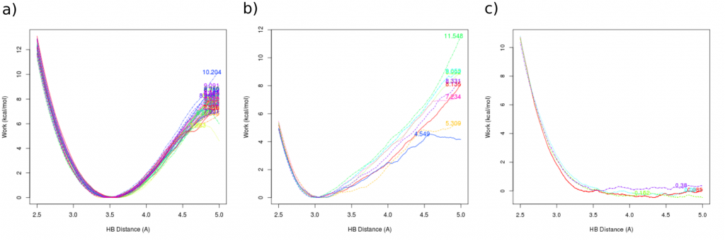
Work value can be calculated for all of the trajectories. The main result (WQB) is the lowest value of work calculated from all of trajectories, printed in file wqb_final.txt.
wqb_plot.png – plot generated at the and of DUck simulation, presenting WQB in the function of distance.
A few examples of potential outcomes are presented below. The left (a) shows results for strongly binding ligand. The middle plot (b) shows different outcomes of simulation for a single ligand. Different WQB values are results of different starting states and different trajectories. In the last case (c) ligand is not binding to the chunk and no work is needed to pull it out of the pocket.
In case plots want to be generated manually run command:
Rscript getWqbValues.R plot
Detailed data for SMD is collected in DUCK_*/ and DUCK_325K_*/ folders, divided by temperature and step of simulation. The folders contain files with trajectories. File duck.dat contains four columns: position of the end of string, position of the reference atom in the ligand, force applied to the string to equilibrate pulling of the ligand, work calculated from the force.
Support
If you are having trouble regarding usage of DUck you can ask for support:
Posted by: Maciej Majewski